There are two types of people for those who love Excel and those who don’t know it that much yet. Sorry to start so bluntly, but I’ve really thought for a long time that the most useful type of application is spreadsheets. And no, this is not an argument against the others: word processors, databases, audio and video editing software, collection managers… the list of types of software that I find sensational is very, very long, but if I had to stick to just one (plus web browser, ok, I admit that), I think Excel would be the choice.

A few years ago, Microsoft CEO Satya Nadella declared that Excel was the best Microsoft product ever created, which is a pretty bold statement given the company’s entire history, but also a pretty clear sign the importance attached to the table at Redmond that it was able to dethrone Lotus 1-2-3, just as Word did WordPerfect (which you may be surprised still exists and is sold by Corel), making Microsoft Office a major (though obviously not unique) exponent. solutions for office automation.

Excel is an application that Its goal is to offer countless options, but at the same time to be friendly to practically all types of users., a challenge that can generally be accomplished quite easily. However, this leads to many features being unknown to many users who resort to alternative and less practical means of obtaining results that are actually much more readily available.

If you’re a professional Excel user, it’s quite likely that you already know some or all of them, but if not, I believe you will find among these three Excel trickswhich is actually just a small part of the huge amount of features available in what is, for Satya Nadella and me, Microsoft’s best product to date.

Get tables from the web

A fairly common operation when working with Excel is the transfer of data from a table published on the Internet to a workbook. The most common, if small, is to manually rewrite the values. However, once it grows in size, the most common thing that is usually seen almost always is to copy (Control + C) the table in the source site and later paste it into Excel (Control + V), although in many cases the data is not inserted correctly, some may be lost, etc., requiring careful review and subsequent manual adjustments.

The good news is that Excel actually has a web data import tool that makes these operations much easier. Let’s look at an example:

Imagine you want an Excel document with tables of the elements of the periodic table. An internet search takes you to Wikipedia, which, as you’d expect, has such information (tables grouped by their natural state can be found at the bottom of the article).

Copy the URL of the spreadsheet page you want to transfer to Excel, then go to the application and in the target spreadsheet, select “Data” from the top menu, then click “From Web” , so a new dialog labeled “From Web” will open.

Paste the URL of the data source page into the field in the middle section, then click the “Accept” button. Next, if this is the first time you are getting data from this source, the wizard will ask you what kind of access you want to use. Since we are talking about a public site, you can leave it in default mode, anonymous, and continue. After that, Excel will start analyzing the web page you selected and at the end it will show you a window like this:

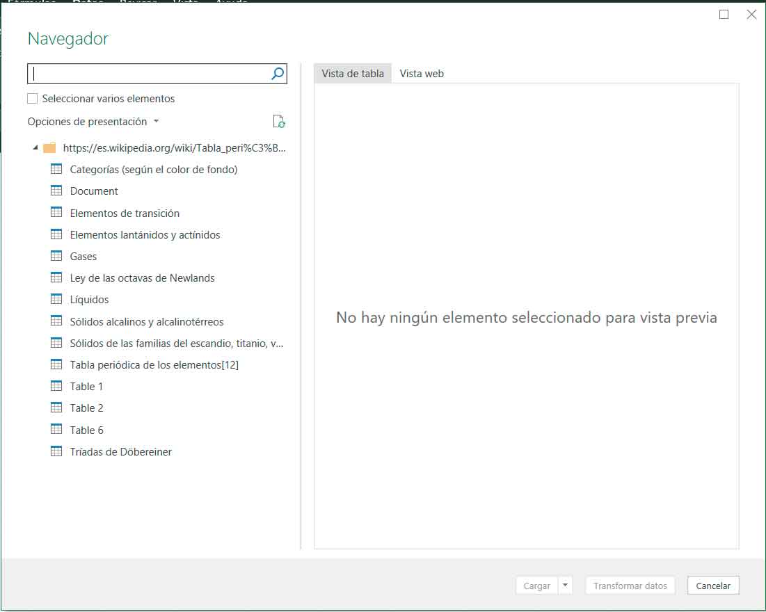
As you can see, all the tables found on this page are displayed on the left, and if you select one of them, its preview will appear on the right:

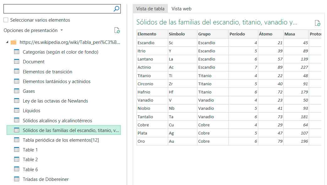
As you can see, a selector is displayed in the list of web tables where you can indicate whether you want to import more than one table. If so, mark it and that way you can select all the ones you want.

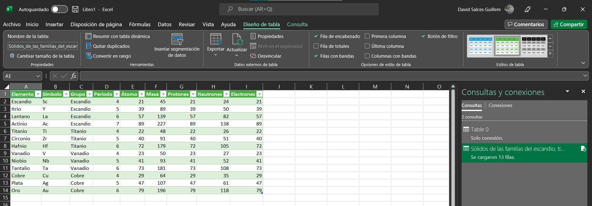
If you want to make changes to the way the data is imported, clicking the “Transform data” button opens an editor where you can define these changes. But if you don’t want to apply the changes, if you want to transfer them from the web to Excel as they are, just click the “Load” button and voila! You will already have the imported data in your Excel sheet along with a set of tools that will offer you more functions related to said import:

Correct the columns or rows

Excel allows you to work with large, very large, monstrously large and inhumanly large tables. And in general, any table worth its salt has a header in the top row and items that are defined in the first column and expanded in subsequent ones. The problem is that, as a general rule, Excel’s display does not take into account that the first row and first column must always remain visible. And that in many cases means that we are constantly scrolling left and up in tables to confirm that we are editing the correct cell. Poorly.

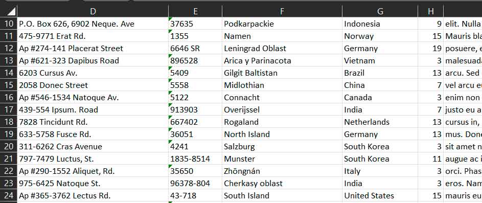
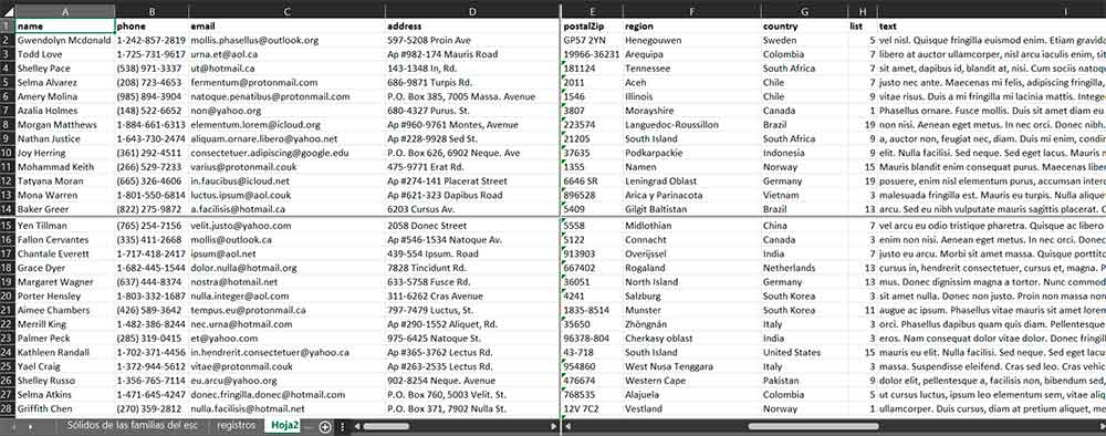
Let’s say you’re working on a table like this (don’t worry, the data shown in it isn’t real, it was randomly generated in GenerateData):

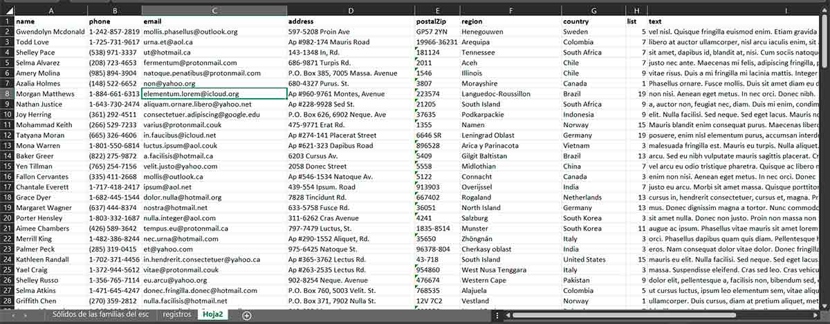
Once you start scrolling down to lower records, the headers indicating what type of data is displayed in each column will no longer be visible. And if you scroll to the right, you’ll see more data for each record, but you’ll lose sight of the name that lets you identify which person corresponds to which data:

To end this problem, just go to the “Data” section in the top menu and after viewing its options, click “Freeze” to display the menu.

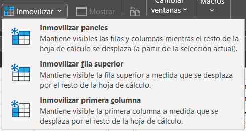
As you already deduced, you will only have to select its second or third entry, depending on what you want to be permanently displayed (you can only select one of the two), and this way you will be able to move around the sheet without losing an overview of the headings or dates in the first column.

And what happens if you don’t want to choose between row or column, but always have both visible? Don’t worry, there is a solution too. Instead of using the freeze function, you will see that there is also “Split” in the same function box. Click on it and at that moment you will see how the view of the sheet is divided into four parts:

Then place the mouse pointer directly over the four quadrant split so that it changes to a four point cursor, click and drag until the split looks like this:

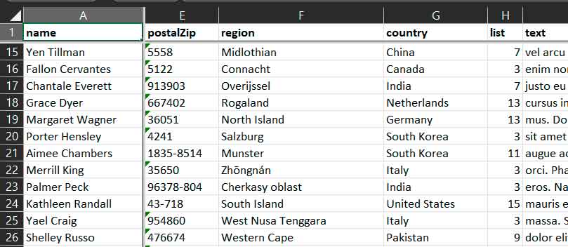
Then click on any of the cells in the central quadrant and you will be able to move around the entire sheet without losing sight of the first row or first column of the document.

Change the axis data

Sometimes, when we start designing an Excel table or adding data, we are not completely clear about its organization, that is, how we want to arrange it horizontally and vertically. This leads to the fact that if we do not take into account the development that said document can have as it grows, that at some point we see that we are wrong. Let’s look at an example.

Imagine that you are the chairman of your community (I feel sorry for you in that case) and that you create a document to track the payments of the community residents. At first, it seems to you that it is most practical to put apartments in the first column, and payments (or lack thereof) are recorded in the following ones. The end result would be something like this:

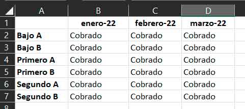
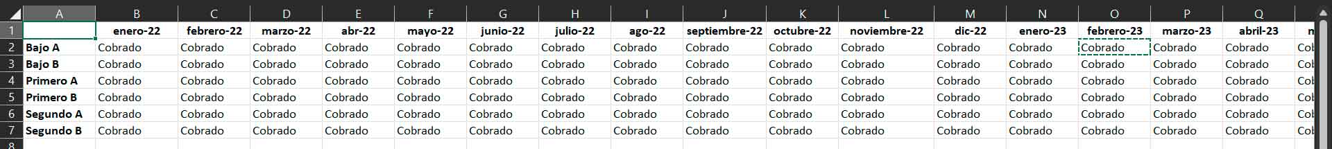
It looks good from this point of view… the problem is that as time goes on and new moons arrive, the result will be much worse, right?

No, don’t even start thinking about copying the data to a new sheet with the correct orientation, that would be quite a difficult process and quite easy to make mistakes. Don’t worry, Excel has a specific function for data transposition. To use it, select all the data you want to reorient and press Control + C to copy it to the Windows clipboard.

Then place the mouse pointer in the place where you want to insert them (for this purpose in the upper left corner of the range of cells) already with a new orientation, click on this cell with the right mouse button, click on the item ” Paste differently” from the context menu and in the window that will be displayed

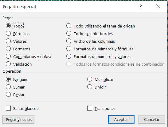
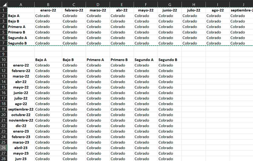
Make sure you check “Transponder” and click “OK”. In this way, the data will be copied automatically already with the new orientation: