


Calculate percentages using Excel
- July 31, 2022
- 0
There are many people there for whom calculating percentages is an uphill climb. And it is that, although it is a simple operation, it is common to see


9621 Agnes Crossing, Lake Suzanneview, New Mexico Island 84604-9295.
There are many people there for whom calculating percentages is an uphill climb. And it is that, although it is a simple operation, it is common to see

There are many people there for whom calculating percentages is an uphill climb. And it is that, although it is a simple operation, it is common to see errors in the formulas for its calculation. I won’t name names, but I’ve also come across errors of this type on professional websites that are supposed to help people who have problems with them. I know that may sound exaggerated, but I guarantee you it’s true.
Fortunately, we once again have Excel, an application that is used for almost everything and that many of us consider essential every day. And yes, it’s true that there are many operations that can be performed with a normal calculator, such as the one included in Windows or found on our smartphones (and calculating percentages is among them), but why not go a little further ? We will see three common operations related to percentagesand create a table that will allow us to calculate them automatically.
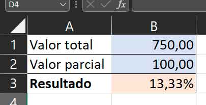
This is obviously the easiest of the three calculators. With it, we are looking for the sum and percentage to be entered, and the calculator will return a numerical value. Perhaps this is better understood with an example: if I enter 200 as a sum and 5% as a percentage, the calculator returns 10 because 10 is 5% of 200.
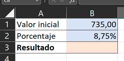
Let’s start with the visual design of the calculator. In my case, I like to use colors to distinguish which cells we have to enter data into and which ones we don’t. We can also block the cells in which the formulas will be contained so that we do not delete them by mistake, we will tell you how to do it in the next practical. Anyway, after applying formats and such, my calculator looks like this:
As you can deduce, we will need to enter the sum in B1 and the percentage in B2. However, do not forget to use the appropriate formats for these cells, i.e. a number in B1 and B3 and a percentage in B2:
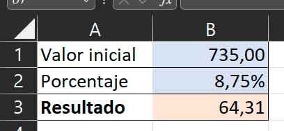
Now just go to B3 and type the following formula: “=B1*B2” (without quotes). And that’s all. With this simple formula, you’ll already have a basic percentage calculator:
Remember, yes, change the cell references if you use other than the ones shown in the images.
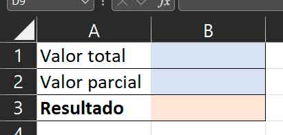
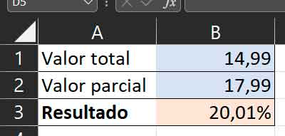
Let’s turn the situation around. Imagine you want to enter two numbers and the calculator tells you what the percentage of B is with respect to A. Again with the example that if you tell A to be 200 and B to be 80, the calculator will tell you that 80 is 40% of 200 .
As with the previous one, make its visual design, in my case it is the following:
Of course, in this case you will need to apply a number format to cells B1 and B2 and a percentage to B3. With all this ready, go to B3 and type the formula “=1/B1*B2” (again without the quotes of course) and the calculator will be ready:
Note that in the example, the B value is lower than the A value, but in reality it can be used the other way around, for example to calculate the percentage increase in price. For this, you can remember to subtract 100 from the result, or you can use this modified version of the formula: “=(1/B1*B2)-1”.
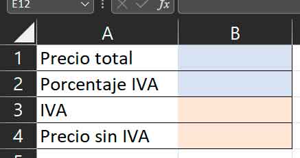
Imagine that you have paid for a product or service and you only know the final amount that you had to pay, but you do not know how much of it corresponds to VAT. The good news is that if you know what rate was used, calculating it is very easy. Recall that in Spain there are these three types of VAT:
| VAT rate | Tax rate |
| General | 21.00% |
| Reduced | 10.00% |
| super reduced | 4.00% |
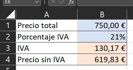
And what we want is a calculator that will give us the final price we paid and the corresponding VAT rate, and it will give us as an answer what we paid as the rate and the amount excluding VAT. So in this case we will use two input fields and two output fields, something like this:
In this case, we will apply the currency format to cells B1, B3, and B4 and the percentage format to cell B2. When everything is ready, we write the formula “=(B1/(1+B2))*B2” in cell B3 and then “=B1-B3” in cell B4. So when we enter the corresponding values in B1 and B2, we can see the VAT breakdown:
As you can see, performing this type of operation is really easy with Excel. And if you want to see more of Microsoft’s spreadsheet tricks, here are three more that might come in handy for you.
Source: Muy Computer

Alice Smith is a seasoned journalist and writer for Div Bracket. She has a keen sense of what’s important and is always on top of the latest trends. Alice provides in-depth coverage of the most talked-about news stories, delivering insightful and thought-provoking articles that keep her readers informed and engaged.


